References:
Bach et al. (2015), Samek et al. (2016), Ancona et al. (2017), Dabkowski and Gal (2017), Shrikumar et al. (2017), Chattopadhay et al. (2018), Chu et al. (2018), Guo et al. (2018b), Guo et al. (2018a), Liu et al. (2018b), Nguyen (2018), Petsiuk (2018), Wang et al. (2018b), Yang et al. (2018b), Annasamy and Sycara (2019), Arya et al. (2019), Brahimi et al. (2019), DeYoung et al. (2019), Fong et al. (2019), Kanehira et al. (2019), Kapishnikov et al. (2019), Lin et al. (2019), Pope et al. (2019), Schlegel et al. (2019), Serrano and Smith (2019), Wagner et al. (2019), Yuan et al. (2019), Ayush et al. (2020), Brunke et al. (2020), Carton et al. (2020), Chen et al. (2020), Cong et al. (2020), Fan et al. (2020), Hsieh et al. (2020), Nguyen et al. (2020), Pan et al. (2020b), Rieger and Hansen (2020), Schlegel et al. (2020), Schulz et al. (2020), Singh et al. (2020), Wang et al. (2020a), Warnecke et al. (2020), Shawi et al. (2021), Ge et al. (2021b), Jethani et al. (2021), Jung and Oh (2021), Liu et al. (2021b), Luss et al. (2021), Poppi et al. (2021), Singh et al. (2021), Situ et al. (2021), Sun et al. (2021), Velmurugan et al. (2021a), Velmurugan et al. (2021b), Vu et al. (2021), Wang et al. (2021), Yin et al. (2021), Albini et al. (2022), Atanasova et al. (2022), Dai et al. (2022), Silva et al. (2022), Funke et al. (2022), Hameed et al. (2022), Müller et al. (2022), Ngai and Rudzicz (2022), Rong et al. (2022), Tan et al. (2022), Veerappa et al. (2022), Šimić et al. (2022), Zou et al. (2022), Agarwal et al. (2023), Alangari et al. (2023a), Jin et al. (2023), Schlegel and Keim (2023), Awal and Roy (2024)
Toggle Text Reference
A common and versatile strategy for evaluating explanation quality is to assess how perturbing features based on the explanans affects model predictions. This approach captures both the necessity (correctness) and sufficiency (completeness) of features highlighted by an explanans [Carton et al. (2020), DeYoung et al. (2019), Alangari et al. (2023a)]. Details on perturbation strategies are outlined in Perturbation Strategies.
Perturbation Scope: Perturbations can be applied either in a fixed-size or iterative manner. Fixed-size perturbations change a predefined amount of information at once [Guo et al. (2018a), DeYoung et al. (2019), Warnecke et al. (2020), Jethani et al. (2021), Jung and Oh (2021), Velmurugan et al. (2021a), Velmurugan et al. (2021b), Wang et al. (2021), Silva et al. (2022), Agarwal et al. (2023)]. The amount of removed features can be selected as a fixed number [Bach et al. (2015), Samek et al. (2016), Ancona et al. (2017), Chu et al. (2018), Schlegel et al. (2019), Nguyen et al. (2020), Alangari et al. (2023a), Schlegel and Keim (2023)] or based on a threshold over cumulative importance scores [Brahimi et al. (2019), Pope et al. (2019), Schlegel et al. (2019), Ngai and Rudzicz (2022), Schlegel and Keim (2023)]. Iterative perturbation gradually removes features one by one or in batches [Bach et al. (2015), Samek et al. (2016), Ancona et al. (2017), Petsiuk (2018), DeYoung et al. (2019), Rieger and Hansen (2020), Jin et al. (2023)].
Perturbation Order: The order in which features are perturbed is critical. Most relevant first (MoRF) evaluates correctness: removing the most important features should lead to a sharp performance drop if the explanation correctly highlights necessary features [Bach et al. (2015), Samek et al. (2016), Chu et al. (2018), DeYoung et al. (2019), Pope et al. (2019), Schlegel et al. (2019), Carton et al. (2020), Rieger and Hansen (2020), Ngai and Rudzicz (2022), Alangari et al. (2023a), Jin et al. (2023), Schlegel and Keim (2023)]. Least relevant first (LeRF) tests completeness: performance should remain high if unimportant features are removed first [Bach et al. (2015), Ancona et al. (2017), Dabkowski and Gal (2017), Guo et al. (2018a), Annasamy and Sycara (2019), DeYoung et al. (2019), Wagner et al. (2019), Carton et al. (2020), Singh et al. (2020), Wang et al. (2020a), Jethani et al. (2021), Liu et al. (2021b), Singh et al. (2021), Wang et al. (2021), Dai et al. (2022), Silva et al. (2022), Alangari et al. (2023a)]. Alternatively, some authors reverse the entire process by starting from a blank input and adding features incrementally [Petsiuk (2018), Arya et al. (2019), Kapishnikov et al. (2019), Luss et al. (2021), Situ et al. (2021), Sun et al. (2021), Atanasova et al. (2022), Funke et al. (2022), Tan et al. (2022)], which is functionally equivalent, with MoRF addition corresponding to LeRF deletion, and vice-versa (for an illustration see the figure below).
Measure Score: The performance change is measured using various scoring mechanisms. These include raw prediction difference [Bach et al. (2015), Chu et al. (2018), DeYoung et al. (2019), Kapishnikov et al. (2019), Chen et al. (2020), Cong et al. (2020), Schulz et al. (2020), Ngai and Rudzicz (2022)], normalized or relative variants [Chattopadhay et al. (2018), Kapishnikov et al. (2019), Schulz et al. (2020), Jung and Oh (2021), Velmurugan et al. (2021a), Velmurugan et al. (2021b), Ngai and Rudzicz (2022)], or evaluation of loss and accuracy metrics [Bach et al. (2015), Chu et al. (2018), Kapishnikov et al. (2019), Lin et al. (2019), Schlegel et al. (2019), Serrano and Smith (2019), Wagner et al. (2019), Warnecke et al. (2020), Sun et al. (2021), Wang et al. (2021), Silva et al. (2022), Schlegel and Keim (2023)]. Some works use statistical distances such as Kullback-Leibler divergence [Liu et al. (2021b), Agarwal et al. (2023)], Kendall's Tau [Singh et al. (2020), Singh et al. (2021)], or Pearson correlation [Poppi et al. (2021)].
Aggregation: For iterative perturbations, the results can be aggregated as the average performance change [Samek et al. (2016), Ancona et al. (2017)], the area over the perturbation curve (AOPC) [Samek et al. (2016), Brahimi et al. (2019), DeYoung et al. (2019), Rieger and Hansen (2020)], or the area under it (AUPC) [Petsiuk (2018), Ngai and Rudzicz (2022), Šimić et al. (2022), Jin et al. (2023)]. The area between MoRF and LeRF (ABPC) may also be computed [Nguyen et al. (2020), Schulz et al. (2020)], optionally with decay weighting to emphasize early changes [Šimić et al. (2022)].
Baselines: To contextualize results, explanation can be compared against various baselines, including random feature selections [Samek et al. (2016), Schlegel et al. (2019), Schlegel and Keim (2023), Serrano and Smith (2019), Jin et al. (2023)], zero-inputs [Schulz et al. (2020)], or naïve explanation such as edge detectors [Hooker et al. (2019)]. Advanced setups may compare against models trained on random labels or with inserted irrelevant features to bound the quality of explanation [Hameed et al. (2022)].
Variants:
• Evaluating explanantia across all classes per instance, not only the predicted class [Pope et al. (2019), Awal and Roy (2024)].
• Sanity checks verifying whether the perturbation curve behaves monotonically [Arya et al. (2019), Fong et al. (2019), Luss et al. (2021)], or whether MoRF always performs worse than LeRF [Šimić et al. (2022)].
• Normalizing the performance drop by the input difference to mitigate distribution shift: [Ge et al. (2021b), Schlegel and Keim (2023)].
• Plotting performance over remaining entropy rather than number of perturbed features [Kapishnikov et al. (2019)].
• Training with randomized feature masking to improve model stability, although this may reduce causality fidelity [Jethani et al. (2021)].
Alternatives: Further, we may change the perspective through alternative formulations:
• Counting the minimum number of features needed to change the model's prediction (in MoRF deletion) [Nguyen (2018)] or using differences between class-specific explanantia to guide perturbations [Shrikumar et al. (2017)].
• Treating perturbed inputs as counterfactuals and applying metrics such as Minimality (see Metric “Minimality”) [Fan et al. (2020), Ge et al. (2021b), Albini et al. (2022)].
• Replacing fixed perturbations with adversarial optimization over features to evaluate minimum change necessary for altering predictions [Hsieh et al. (2020), Vu et al. (2021)].
The approach may be extended to CEs by either mapping concepts to features (e.g., concept-based saliency maps by [Lucieri et al. (2020)]), or perturbing internal activations at the concept layer [Shawi et al. (2021)].
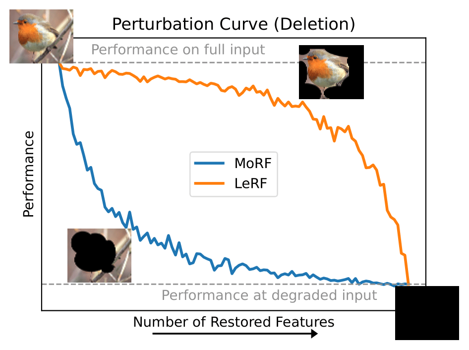
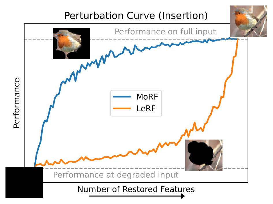
Examples for ideal Perturbation Curves to evaluate feature attributions. Insertion and Deletion approaches are equivalent when switching MoRF for LeRF ordering and vice versa. Deletion MoRF (Insertion LeRF) can be used to evaluate correctness, and Insertion MoRF (Deletion LeRF) to evaluate completeness.